Introduction & Problem Scenario
Original Paper: “Auto-Encoding Variational Bayes” by Diederik P. Kingma and Max Welling (2013) arXiv: 1312.6114
The Central Question
The paper opens with a fundamental question:
“How can we perform efficient inference and learning in directed probabilistic models, in the presence of continuous latent variables with intractable posterior distributions, and large datasets?”
This single sentence contains the entire motivation for VAEs. It’s dense with technical terms — let’s break down every piece.
Breaking Down the Question
”Efficient inference and learning”
Learning = figuring out the rules of a system from examples.
- Example: You show a model 50,000 images of handwritten digits. Learning means the model discovers what makes a “7” look like a “7” — the strokes, angles, proportions.
Inference = using those learned rules to answer questions about new data.
- Example: Given a new handwritten digit, inference asks: “What hidden factors produced this specific image?” Maybe: thick stroke style, slight rightward slant, written quickly.
Efficient = doing both of these fast enough to be practical.
- Training on millions of images shouldn’t take years
- Inference on a single image shouldn’t take minutes
”Directed probabilistic models”
A probabilistic model treats data as random outcomes governed by probability distributions, not fixed rules.
- Example: Instead of saying “a 7 always has this exact shape,” we say “a 7 is likely to have a vertical stroke and a horizontal bar, with some random variation.”
Directed means the model has a clear cause → effect flow (like a flowchart):
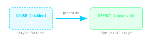 The directed model: hidden causes (z) generate observable effects (x). The causation flows one direction.
Example: The hidden “intent to write a 7 in a rushed style” causes the specific pixels you see. The causation flows one direction: hidden → visible.
”Continuous latent variables”
Latent = hidden. These are factors that exist but we never directly see.
- Example: When you look at a handwritten “3”, you don’t see the writer’s mood, their pen angle, or how fast they wrote. But those hidden factors influenced the result.
Variables = quantities that can take different values.
Continuous = the variables can be any real number, not just categories.
- Discrete: “The digit is a 0, 1, 2, … or 9” (10 options)
- Continuous: “The slant angle is 12.7 degrees” (infinite options between any two values)
Why continuous is harder: With 10 discrete options, you can check each one. With continuous variables, there are infinitely many possibilities — you can’t enumerate them.
”Intractable posterior distributions”
Let’s break this into three parts:
Distribution = a mathematical description of how likely different outcomes are.
- Example: “There’s a 30% chance the hidden style is ‘neat’ and 70% chance it’s ‘messy’”
Posterior = the distribution over hidden causes after you’ve seen the evidence.
- Before seeing the image: “Any writing style is possible” (this is the prior)
- After seeing a messy “5”: “Given this messy image, what writing style likely produced it?” (this is the posterior)
In math: $p(\text{hidden} | \text{observed})$ — read as “probability of hidden stuff, given what we observed”
Intractable = mathematically impossible to compute exactly.
Here’s why it’s intractable: To compute the posterior, you need to use Bayes’ rule:
$$p(\text{hidden}|\text{observed}) = \frac{p(\text{observed}|\text{hidden}) \times p(\text{hidden})}{p(\text{observed})}$$
That denominator $p(\text{observed})$ requires summing over every possible hidden state:
$$p(\text{observed}) = \int_{\text{all possible hidden states}} p(\text{observed}|\text{hidden}) \times p(\text{hidden}) , d(\text{hidden})$$
With continuous, high-dimensional hidden variables and a neural network involved, this integral has no closed-form solution. You’d need infinite compute to calculate it exactly.
”Large datasets”
This means millions of training examples (like ImageNet with 14 million images, or datasets of millions of faces).
Why it’s a challenge: Many traditional methods require expensive computations per datapoint. If each image needs 10 seconds of processing, a million images would take 115 days — just for one pass through the data!
The paper wants methods that:
- Use minibatches (process 100 images at a time, not all million)
- Scale linearly (2× more data = 2× more time, not 4× or worse)
- Work with stochastic gradient descent (the workhorse of deep learning)
The Full Question, Translated
Original:
“How can we perform efficient inference and learning in directed probabilistic models, in the presence of continuous latent variables with intractable posterior distributions, and large datasets?”
Plain English:
“How do we quickly train models that assume hidden continuous factors cause our observations, when we mathematically can’t compute what those hidden factors are, and we have millions of training examples?”
The VAE paper’s answer: Use neural networks to approximate what we can’t compute exactly, and design everything so standard deep learning tools (backpropagation, SGD) just work.
The Generative Model Setup
Consider a dataset $\mathbf{X} = {\mathbf{x}^{(i)}}_{i=1}^{N}$ consisting of $N$ i.i.d. samples. The paper assumes this data was generated by some random process involving an unobserved continuous random variable $\mathbf{z}$:
- A value $\mathbf{z}^{(i)}$ is generated from some prior distribution $p_{\theta^*}(\mathbf{z})$
- A value $\mathbf{x}^{(i)}$ is generated from some conditional distribution $p_{\theta^*}(\mathbf{x}|\mathbf{z})$
Let’s Decode This Step by Step
The Dataset
$\mathbf{X} = {\mathbf{x}^{(i)}}_{i=1}^{N}$ just means: “We have N data samples, labeled 1 through N”
- $\mathbf{x}^{(1)}$ = first sample (e.g., first image)
- $\mathbf{x}^{(2)}$ = second sample
- …
- $\mathbf{x}^{(N)}$ = last sample
Example: If you have 50,000 images of handwritten digits, then N = 50,000, and $\mathbf{x}^{(3721)}$ is the 3,721st image.
”i.i.d.” (Independent and Identically Distributed)
This is a common assumption meaning:
- Independent: Knowing one sample tells you nothing about another (image #500 doesn’t affect image #501)
- Identically distributed: All samples come from the same underlying process (all are handwritten digits, not a mix of digits and cats)
The Hidden Story Behind Each Data Point
The paper imagines that nature generated each image through a two-step process:
Step 1: Pick a “recipe” from the prior
$$\mathbf{z}^{(i)} \sim p_{\theta^*}(\mathbf{z})$$
“Sample a hidden code $\mathbf{z}$ from the prior distribution”
In plain English: Before drawing a digit, nature first randomly decides the “style settings”:
- How thick should the stroke be?
- What angle/slant?
- How loopy vs angular?
- Written fast or carefully?
These hidden settings are the latent variable $\mathbf{z}$. The prior $p(\mathbf{z})$ describes how likely each combination of settings is before we see any specific image.
Step 2: Generate the actual image from that recipe
$$\mathbf{x}^{(i)} \sim p_{\theta^*}(\mathbf{x}|\mathbf{z})$$
“Sample the visible data $\mathbf{x}$ given the hidden code $\mathbf{z}$”
In plain English: Given those style settings, nature “renders” the actual pixels you see. The same recipe might produce slightly different images (randomness in the exact pixel values), but they’d all have similar style.
What Does the $\theta^*$ Mean?
$\theta^*$ represents the true parameters — the actual rules nature uses to generate data.
Think of it as the “ground truth settings” of the universe’s image-generation machine. We don’t know these parameters; we’re trying to learn an approximation $\theta$ that gets close to $\theta^*$.
A Concrete Example
Imagine nature generating a handwritten “7”:
-
Prior sampling: Nature picks $\mathbf{z} = [0.8, -0.3, 0.5, …]$
- These numbers encode: “thick stroke, slight left slant, medium speed, …”
-
Conditional generation: Given those settings, nature produces a specific 28×28 pixel image
- The decoder $p(\mathbf{x}|\mathbf{z})$ turns the abstract code into concrete pixels
The key insight: We only ever see the final image $\mathbf{x}$. We never see the hidden code $\mathbf{z}$ that produced it. That’s why it’s called a latent (hidden) variable.
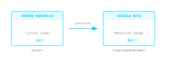 The generative process: latent codes z are sampled from the prior p(z), then transformed through the decoder p(x|z) to produce observable data x.
Crucially: The true parameters $\theta^*$ and the latent variables $\mathbf{z}^{(i)}$ are unknown to us. We only observe the final outputs $\mathbf{x}^{(i)}$. The goal is to reverse-engineer both:
- What are the hidden codes $\mathbf{z}$ for each image?
- What are the rules $\theta$ that govern the generation process?
The Three Intractability Problems
The paper explicitly states they do NOT make common simplifying assumptions. They want an algorithm that works even when:
Problem 1: Intractable Marginal Likelihood
The marginal likelihood (also called “evidence”) is:
$$p_\theta(\mathbf{x}) = \int p_\theta(\mathbf{z}) p_\theta(\mathbf{x}|\mathbf{z}) , d\mathbf{z}$$
This integral sums over ALL possible values of the latent variable $\mathbf{z}$. For a neural network decoder $p_\theta(\mathbf{x}|\mathbf{z})$, this integral has no closed-form solution.
Why it matters: We can’t evaluate or differentiate the marginal likelihood directly.
Problem 2: Intractable True Posterior
Given an observation $\mathbf{x}$, what latent code $\mathbf{z}$ generated it? By Bayes’ rule:
$$p_\theta(\mathbf{z}|\mathbf{x}) = \frac{p_\theta(\mathbf{x}|\mathbf{z}) p_\theta(\mathbf{z})}{p_\theta(\mathbf{x})}$$
But the denominator $p_\theta(\mathbf{x})$ is the intractable marginal likelihood from Problem 1!
Why it matters:
- The EM algorithm requires computing/sampling from the true posterior — can’t use it
- Mean-field variational Bayes requires tractable expectations — also can’t use it
Problem 3: Large Datasets
Even if we could approximate these integrals with sampling (e.g., Monte Carlo methods):
- We have millions of datapoints
- Each would require an expensive sampling loop
- Batch optimization becomes prohibitively slow
What They Want to Achieve
The paper proposes solutions to three related problems:
| Problem | Goal | Application |
|---|---|---|
| Parameter estimation | Learn $\theta$ via approximate ML/MAP | Understanding the data-generating process; generating new data |
| Posterior inference | Given $\mathbf{x}$, infer $\mathbf{z}$ | Coding, compression, representation learning |
| Marginal inference | Compute $p(\mathbf{x})$ | Denoising, inpainting, super-resolution |
The Key Insight: The Recognition Model
The paper’s solution introduces a recognition model $q_\phi(\mathbf{z}|\mathbf{x})$: an approximation to the intractable true posterior $p_\theta(\mathbf{z}|\mathbf{x})$.
Critical difference from traditional variational inference:
- Traditional mean-field VI: $q$ is factorial, parameters computed from closed-form expectations
- VAE approach: $q_\phi(\mathbf{z}|\mathbf{x})$ is parameterized by a neural network with parameters $\phi$
The parameters $\phi$ are learned jointly with the generative model parameters $\theta$.
Encoder-Decoder Interpretation
From a coding theory perspective:
| Component | Probabilistic View | Coding View |
|---|---|---|
| $q_\phi(\mathbf{z} | \mathbf{x})$ | Approximate posterior |
| $p_\theta(\mathbf{x} | \mathbf{z})$ | Likelihood |
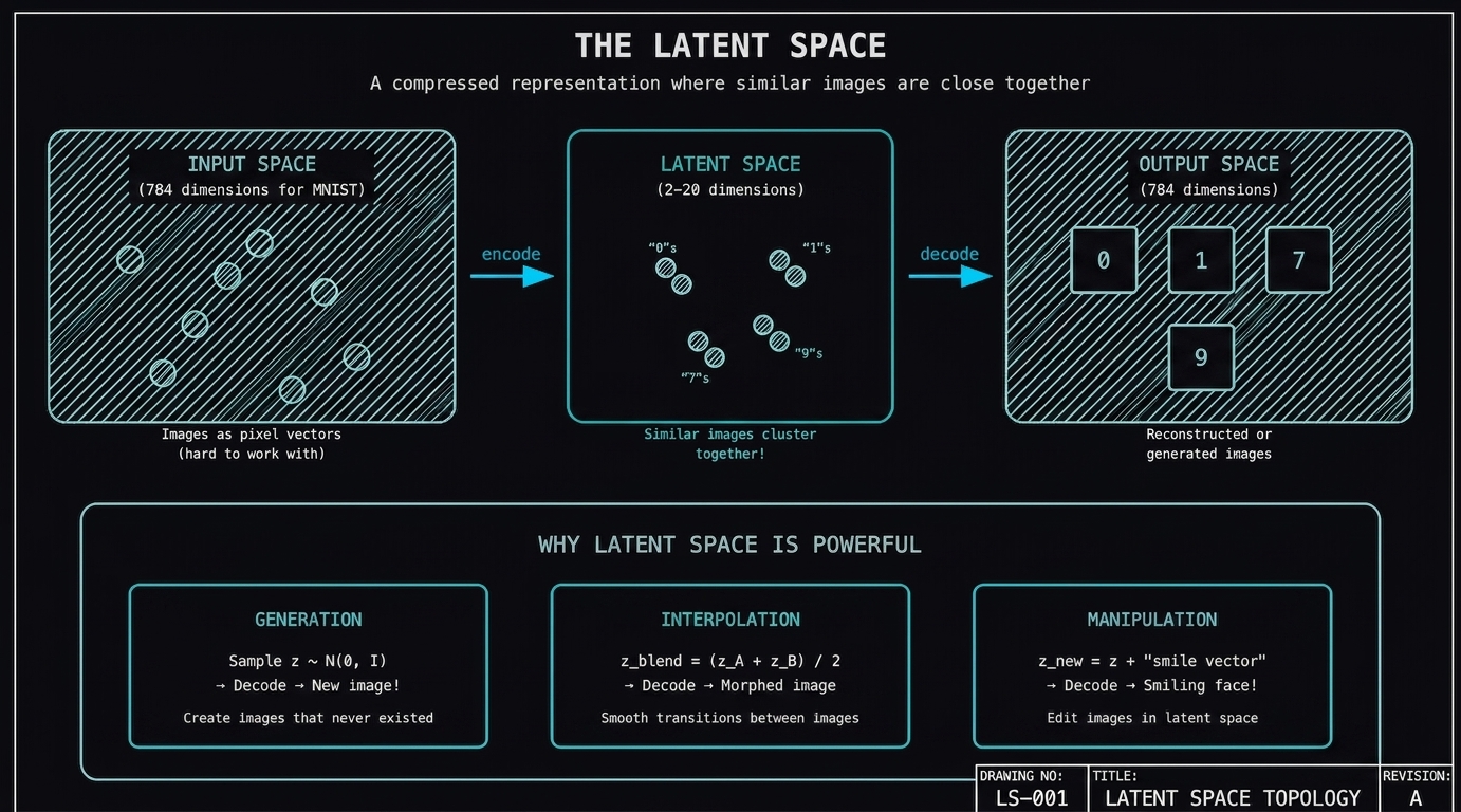 The latent space is a compressed representation where similar data points cluster together. This diagram shows how high-dimensional input data (left) gets encoded into a low-dimensional latent space (center), then decoded back to output space (right).
The Graphical Model
The paper presents this as a directed graphical model (Figure 1 in paper):
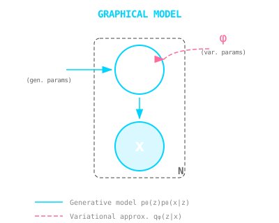 The VAE graphical model. Solid lines show the generative model p(z)p(x|z), while dashed lines show the variational approximation q(z|x). The plate notation (N) indicates this structure repeats for each datapoint.
Summary: The Setup
Before diving into the solution, here’s what we have:
- Data: $\mathbf{X} = {\mathbf{x}^{(i)}}_{i=1}^{N}$ (e.g., images)
- Latent variables: $\mathbf{z}$ (hidden “codes” for each datapoint)
- Prior: $p_\theta(\mathbf{z})$ (typically $\mathcal{N}(\mathbf{0}, \mathbf{I})$)
- Decoder/Likelihood: $p_\theta(\mathbf{x}|\mathbf{z})$ (neural network)
- Encoder/Approximate posterior: $q_\phi(\mathbf{z}|\mathbf{x})$ (neural network)
- Goal: Learn both $\theta$ and $\phi$ jointly, efficiently, at scale