Appendix: Mathematical Details
This section covers Appendices B and C of the paper: the analytical KL divergence for Gaussians and the specific MLP architectures used.
Appendix B: KL Divergence for Gaussians
One of the key computational advantages of VAEs is that when both the approximate posterior $q_\phi(\mathbf{z}|\mathbf{x})$ and the prior $p(\mathbf{z})$ are Gaussian, the KL divergence has a closed-form solution.
Setup
Let:
- $q_\phi(\mathbf{z}|\mathbf{x}) = \mathcal{N}(\mathbf{z}; \boldsymbol{\mu}, \boldsymbol{\sigma}^2 \mathbf{I})$ — encoder output
- $p(\mathbf{z}) = \mathcal{N}(\mathbf{z}; \mathbf{0}, \mathbf{I})$ — prior (standard Gaussian)
Both have diagonal covariance (independence across dimensions).
The KL Divergence Formula
For two multivariate Gaussians $\mathcal{N}_0 = \mathcal{N}(\boldsymbol{\mu}_0, \boldsymbol{\Sigma}_0)$ and $\mathcal{N}_1 = \mathcal{N}(\boldsymbol{\mu}_1, \boldsymbol{\Sigma}_1)$:
$$D_{KL}(\mathcal{N}_0 | \mathcal{N}_1) = \frac{1}{2} \left( \text{tr}(\boldsymbol{\Sigma}_1^{-1} \boldsymbol{\Sigma}_0) + (\boldsymbol{\mu}_1 - \boldsymbol{\mu}_0)^T \boldsymbol{\Sigma}_1^{-1} (\boldsymbol{\mu}_1 - \boldsymbol{\mu}_0) - J + \log \frac{|\boldsymbol{\Sigma}_1|}{|\boldsymbol{\Sigma}_0|} \right)$$
Where $J$ is the dimensionality of the latent space.
Simplification for VAE Case
For the VAE, we have:
- $\mathcal{N}0 = q\phi(\mathbf{z}|\mathbf{x}) = \mathcal{N}(\boldsymbol{\mu}, \text{diag}(\boldsymbol{\sigma}^2))$
- $\mathcal{N}_1 = p(\mathbf{z}) = \mathcal{N}(\mathbf{0}, \mathbf{I})$
So:
- $\boldsymbol{\mu}_0 = \boldsymbol{\mu}$ (encoder mean)
- $\boldsymbol{\mu}_1 = \mathbf{0}$ (prior mean)
- $\boldsymbol{\Sigma}_0 = \text{diag}(\boldsymbol{\sigma}^2)$ (encoder variance)
- $\boldsymbol{\Sigma}_1 = \mathbf{I}$ (prior variance)
Term-by-Term Derivation
Term 1: Trace
$$\text{tr}(\boldsymbol{\Sigma}_1^{-1} \boldsymbol{\Sigma}0) = \text{tr}(\mathbf{I}^{-1} \cdot \text{diag}(\boldsymbol{\sigma}^2)) = \text{tr}(\text{diag}(\boldsymbol{\sigma}^2)) = \sum{j=1}^{J} \sigma_j^2$$
Term 2: Quadratic (Mahalanobis distance)
$$(\boldsymbol{\mu}_1 - \boldsymbol{\mu}_0)^T \boldsymbol{\Sigma}_1^{-1} (\boldsymbol{\mu}_1 - \boldsymbol{\mu}0) = (\mathbf{0} - \boldsymbol{\mu})^T \mathbf{I} (-\boldsymbol{\mu}) = \boldsymbol{\mu}^T \boldsymbol{\mu} = \sum{j=1}^{J} \mu_j^2$$
Term 3: Log determinant ratio
$$\log \frac{|\boldsymbol{\Sigma}1|}{|\boldsymbol{\Sigma}0|} = \log \frac{|\mathbf{I}|}{|\text{diag}(\boldsymbol{\sigma}^2)|} = \log \frac{1}{\prod{j=1}^{J} \sigma_j^2} = -\sum{j=1}^{J} \log \sigma_j^2$$
Final Result (Appendix B)
Combining all terms:
$$D_{KL}(q_\phi(\mathbf{z}|\mathbf{x}) | p(\mathbf{z})) = \frac{1}{2} \left( \sum_{j=1}^{J} \sigma_j^2 + \sum_{j=1}^{J} \mu_j^2 - J - \sum_{j=1}^{J} \log \sigma_j^2 \right)$$
Rearranging:
$$D_{KL} = -\frac{1}{2} \sum_{j=1}^{J} \left( 1 + \log \sigma_j^2 - \mu_j^2 - \sigma_j^2 \right)$$
Or equivalently (negating for the ELBO):
$$-D_{KL}(q_\phi(\mathbf{z}|\mathbf{x}) | p(\mathbf{z})) = \frac{1}{2} \sum_{j=1}^{J} \left( 1 + \log \sigma_j^2 - \mu_j^2 - \sigma_j^2 \right)$$
Implementation
In code (where logvar = $\log \boldsymbol{\sigma}^2$):
# KL divergence: -0.5 * sum(1 + log(σ²) - μ² - σ²)
KLD = -0.5 * torch.sum(1 + logvar - mu.pow(2) - logvar.exp())
Why logvar.exp() gives $\sigma^2$:
- Network outputs $\log \sigma^2$
- $\exp(\log \sigma^2) = \sigma^2$
Interpretation of Each Term
| Term | Expression | Meaning |
|---|---|---|
| $+1$ | Constant | Baseline |
| $+\log \sigma_j^2$ | Log variance | Encourages larger variance (more uncertainty) |
| $-\mu_j^2$ | Squared mean | Penalizes means far from 0 |
| $-\sigma_j^2$ | Variance | Penalizes variance far from 1 |
Balancing act: The KL term pushes the encoder to output:
- Means close to 0
- Variances close to 1
This keeps the latent space organized around the origin.
Appendix C: MLP Encoder and Decoder
The paper provides specific MLP architectures for the encoder and decoder networks.
Notation
| Symbol | Meaning |
|---|---|
| $D$ | Input dimensionality (e.g., 784 for MNIST) |
| $J$ | Latent space dimensionality |
| $H$ | Hidden layer size |
| $\mathbf{W}$ | Weight matrix |
| $\mathbf{b}$ | Bias vector |
Encoder Architecture
The encoder maps input $\mathbf{x}$ to distribution parameters $(\boldsymbol{\mu}, \log \boldsymbol{\sigma}^2)$:
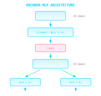 The encoder MLP: input passes through a linear layer and tanh activation, then splits into two heads producing μ and log σ².
Encoder parameters: $\phi = {\mathbf{W}_3, \mathbf{b}_3, \mathbf{W}_4, \mathbf{b}_4, \mathbf{W}_5, \mathbf{b}_5}$
Parameter count:
- $\mathbf{W}_3$: $H \times D$
- $\mathbf{b}_3$: $H$
- $\mathbf{W}_4$: $J \times H$
- $\mathbf{b}_4$: $J$
- $\mathbf{W}_5$: $J \times H$
- $\mathbf{b}_5$: $J$
- Total: $H \cdot D + H + 2 \cdot (J \cdot H + J) = H(D + 1 + 2J) + 2J$
Decoder Architecture (Bernoulli)
For binary data (e.g., MNIST), the decoder outputs Bernoulli probabilities:
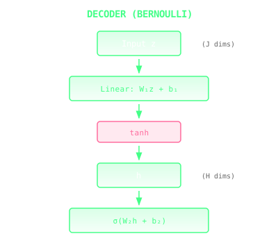 The Bernoulli decoder for binary data: latent z passes through linear + tanh, then linear + sigmoid to produce pixel probabilities.
Decoder parameters: $\theta = {\mathbf{W}_1, \mathbf{b}_1, \mathbf{W}_2, \mathbf{b}_2}$
The output $\mathbf{y}$ represents the probability of each pixel being “on”: $$p_\theta(\mathbf{x}|\mathbf{z}) = \prod_{i=1}^{D} y_i^{x_i} (1 - y_i)^{1-x_i}$$
Decoder Architecture (Gaussian)
For continuous data, the decoder outputs mean and variance. The architecture is similar to Bernoulli but with two output heads (μ and log σ²) instead of a single sigmoid output.
The output distribution: $$p_\theta(\mathbf{x}|\mathbf{z}) = \mathcal{N}(\mathbf{x}; \boldsymbol{\mu}\theta(\mathbf{z}), \text{diag}(\boldsymbol{\sigma}^2\theta(\mathbf{z})))$$
Complete Architecture Diagram
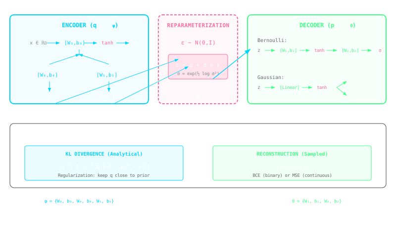 The complete VAE system: encoder produces distribution parameters, reparameterization enables differentiable sampling, decoder reconstructs the input, and the loss combines KL divergence with reconstruction.
Specific Configurations from Paper
MNIST Configuration
| Component | Specification |
|---|---|
| Input dim ($D$) | 784 (28×28 images) |
| Hidden dim ($H$) | 500 |
| Latent dim ($J$) | Varied: 2, 5, 10, 20, 50 |
| Decoder type | Bernoulli (sigmoid output) |
| Activation | tanh |
Total parameters (for $J=50$):
- Encoder: $500 \cdot 784 + 500 + 2 \cdot (50 \cdot 500 + 50) = 442,600$
- Decoder: $500 \cdot 50 + 500 + 784 \cdot 500 + 784 = 418,284$
- Total: ~861K parameters
Frey Face Configuration
| Component | Specification |
|---|---|
| Input dim ($D$) | 560 (28×20 images) |
| Hidden dim ($H$) | 200 |
| Latent dim ($J$) | Varied: 2, 5, 10, 20 |
| Decoder type | Gaussian (outputs μ and σ²) |
| Activation | tanh |
Initialization
The paper uses standard initialization practices:
- Weights: Small random values (typically Gaussian with small std)
- Biases: Zeros or small values
Modern implementations often use:
- Xavier/Glorot initialization for tanh activations
- He initialization for ReLU activations
The Loss Function (Complete)
Combining everything, the total loss for a single datapoint:
$$\text{Loss} = \underbrace{-\frac{1}{2} \sum_{j=1}^{J} \left( 1 + \log \sigma_j^2 - \mu_j^2 - \sigma_j^2 \right)}{\text{KL divergence (analytical)}} \underbrace{- \log p\theta(\mathbf{x}|\mathbf{z})}_{\text{Reconstruction (sampled)}}$$
For Bernoulli Decoder:
$$\text{Loss} = -\frac{1}{2} \sum_{j=1}^{J} \left( 1 + \log \sigma_j^2 - \mu_j^2 - \sigma_j^2 \right) - \sum_{i=1}^{D} \left[ x_i \log y_i + (1-x_i) \log(1-y_i) \right]$$
For Gaussian Decoder (with fixed unit variance):
$$\text{Loss} = -\frac{1}{2} \sum_{j=1}^{J} \left( 1 + \log \sigma_j^2 - \mu_j^2 - \sigma_j^2 \right) + \frac{1}{2} |\mathbf{x} - \boldsymbol{\mu}_\theta(\mathbf{z})|^2$$
Full PyTorch Implementation
import torch
import torch.nn as nn
import torch.nn.functional as F

class VAE(nn.Module):
    """
    Variational Auto-Encoder following the original paper's architecture.
    """
    def __init__(self, input_dim=784, hidden_dim=500, latent_dim=50):
        super(VAE, self).__init__()

        # Encoder layers (φ parameters)
        self.fc3 = nn.Linear(input_dim, hidden_dim)   # W₃, b₃
        self.fc4 = nn.Linear(hidden_dim, latent_dim)  # W₄, b₄ (for μ)
        self.fc5 = nn.Linear(hidden_dim, latent_dim)  # W₅, b₅ (for log σ²)

        # Decoder layers (θ parameters)
        self.fc1 = nn.Linear(latent_dim, hidden_dim)  # W₁, b₁
        self.fc2 = nn.Linear(hidden_dim, input_dim)   # W₂, b₂

    def encode(self, x):
        """
        Encoder: x → (μ, log σ²)
        """
        h = torch.tanh(self.fc3(x))  # Hidden representation
        mu = self.fc4(h)              # Mean
        logvar = self.fc5(h)          # Log variance
        return mu, logvar

    def reparameterize(self, mu, logvar):
        """
        Reparameterization trick: z = μ + σ ⊙ ε
        """
        std = torch.exp(0.5 * logvar)  # σ = exp(½ log σ²)
        eps = torch.randn_like(std)     # ε ~ N(0, I)
        return mu + std * eps

    def decode(self, z):
        """
        Decoder: z → y (Bernoulli probabilities)
        """
        h = torch.tanh(self.fc1(z))
        return torch.sigmoid(self.fc2(h))

    def forward(self, x):
        mu, logvar = self.encode(x)
        z = self.reparameterize(mu, logvar)
        return self.decode(z), mu, logvar


def loss_function(recon_x, x, mu, logvar):
    """
    VAE loss = Reconstruction + KL divergence

    Args:
        recon_x: Reconstructed input (decoder output)
        x: Original input
        mu: Encoder mean
        logvar: Encoder log variance

    Returns:
        Total loss (to be minimized)
    """
    # Reconstruction loss (binary cross-entropy)
    # This is -log p(x|z) for Bernoulli decoder
    BCE = F.binary_cross_entropy(recon_x, x, reduction='sum')

    # KL divergence: -½ Σ(1 + log σ² - μ² - σ²)
    # See Appendix B of paper
    KLD = -0.5 * torch.sum(1 + logvar - mu.pow(2) - logvar.exp())

    return BCE + KLD


# Training loop (simplified)
def train(model, data_loader, optimizer, epoch):
    model.train()
    train_loss = 0

    for batch_idx, (data, _) in enumerate(data_loader):
        data = data.view(-1, 784)  # Flatten MNIST images
        optimizer.zero_grad()

        recon_batch, mu, logvar = model(data)
        loss = loss_function(recon_batch, data, mu, logvar)

        loss.backward()
        train_loss += loss.item()
        optimizer.step()

    return train_loss / len(data_loader.dataset)
Summary
| Appendix | Content | Key Result |
|---|---|---|
| B: KL Divergence | Closed-form for Gaussians | $-\frac{1}{2} \sum_j (1 + \log \sigma_j^2 - \mu_j^2 - \sigma_j^2)$ |
| C: MLP Architecture | Encoder/Decoder specs | Single hidden layer, tanh activation |
These details enable the analytical KL term that gives VAEs their computational efficiency — only the reconstruction term needs Monte Carlo estimation.