The Reparameterization Trick
This section covers Section 2.4 of the paper: the key innovation that enables backpropagation through stochastic sampling.
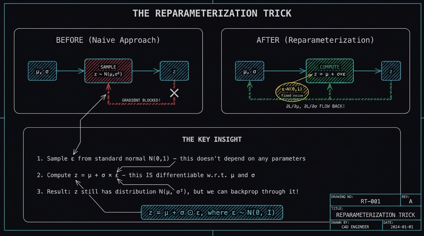 The reparameterization trick solves the gradient problem. BEFORE (left): Sampling directly from N(μ,σ²) blocks gradient flow. AFTER (right): By sampling ε from N(0,1) and computing z = μ + σ×ε, gradients can flow back through μ and σ to train the encoder.
The Problem
During training, we need to:
- Run the encoder to get distribution parameters (e.g., $\boldsymbol{\mu}$ and $\boldsymbol{\sigma}$)
- Sample $\mathbf{z}$ from $q_\phi(\mathbf{z}|\mathbf{x})$
- Run the decoder on $\mathbf{z}$
- Compute the loss
- Backpropagate gradients through the entire computation
The issue: Step 2 involves random sampling. You cannot backpropagate through a random sampling operation!
The sampling operation $\mathbf{z} \sim q_\phi(\mathbf{z}|\mathbf{x})$ is non-differentiable with respect to $\phi$.
The Mathematical Setup
Let $\mathbf{z}$ be a continuous random variable, and let $\mathbf{z} \sim q_\phi(\mathbf{z}|\mathbf{x})$ be some conditional distribution.
Goal: Express $\mathbf{z}$ as a deterministic function of:
- The input $\mathbf{x}$
- The parameters $\phi$
- An auxiliary noise variable $\boldsymbol{\epsilon}$ with a fixed distribution
The Reparameterization
Equation (4):
$$\tilde{\mathbf{z}} = g_\phi(\boldsymbol{\epsilon}, \mathbf{x}) \quad \text{with} \quad \boldsymbol{\epsilon} \sim p(\boldsymbol{\epsilon})$$
Where:
- $p(\boldsymbol{\epsilon})$ is a fixed noise distribution (independent of parameters)
- $g_\phi(\boldsymbol{\epsilon}, \mathbf{x})$ is a differentiable, deterministic function
Key property: If we choose $p(\boldsymbol{\epsilon})$ and $g_\phi$ correctly, then $\tilde{\mathbf{z}}$ has the same distribution as sampling from $q_\phi(\mathbf{z}|\mathbf{x})$.
The Gaussian Case (Most Common)
For a univariate Gaussian $z \sim p(z|x) = \mathcal{N}(\mu, \sigma^2)$:
Reparameterization: $$z = \mu + \sigma \cdot \epsilon \quad \text{where} \quad \epsilon \sim \mathcal{N}(0, 1)$$
Proof that this works:
- $\epsilon \sim \mathcal{N}(0, 1)$ has mean 0, variance 1
- $\sigma \cdot \epsilon$ has mean 0, variance $\sigma^2$
- $\mu + \sigma \cdot \epsilon$ has mean $\mu$, variance $\sigma^2$
- Therefore $z \sim \mathcal{N}(\mu, \sigma^2)$ ✓
For multivariate Gaussian with diagonal covariance $q_\phi(\mathbf{z}|\mathbf{x}) = \mathcal{N}(\mathbf{z}; \boldsymbol{\mu}, \boldsymbol{\sigma}^2 \mathbf{I})$:
$$\mathbf{z} = \boldsymbol{\mu} + \boldsymbol{\sigma} \odot \boldsymbol{\epsilon} \quad \text{where} \quad \boldsymbol{\epsilon} \sim \mathcal{N}(\mathbf{0}, \mathbf{I})$$
Where $\odot$ denotes element-wise multiplication.
Why This Enables Backpropagation
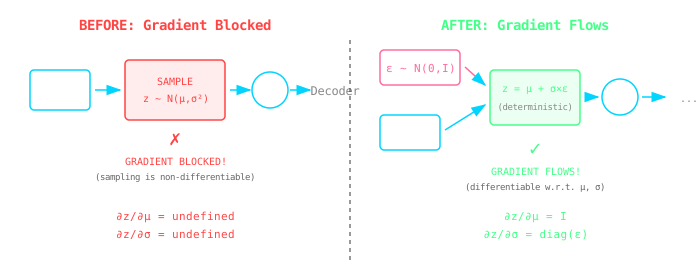 The reparameterization trick transforms a blocked gradient path (left) into a differentiable computation (right) by externalizing the randomness.
Mathematical justification (from the paper):
Given the deterministic mapping $\mathbf{z} = g_\phi(\boldsymbol{\epsilon}, \mathbf{x})$, we know that:
$$q_\phi(\mathbf{z}|\mathbf{x}) \prod_i dz_i = p(\boldsymbol{\epsilon}) \prod_i d\epsilon_i$$
Therefore:
$$\int q_\phi(\mathbf{z}|\mathbf{x}) f(\mathbf{z}) , d\mathbf{z} = \int p(\boldsymbol{\epsilon}) f(\mathbf{z}) , d\boldsymbol{\epsilon} = \int p(\boldsymbol{\epsilon}) f(g_\phi(\boldsymbol{\epsilon}, \mathbf{x})) , d\boldsymbol{\epsilon}$$
And thus:
$$\int q_\phi(\mathbf{z}|\mathbf{x}) f(\mathbf{z}) , d\mathbf{z} \simeq \frac{1}{L} \sum_{l=1}^{L} f(g_\phi(\mathbf{x}, \boldsymbol{\epsilon}^{(l)})) \quad \text{where} \quad \boldsymbol{\epsilon}^{(l)} \sim p(\boldsymbol{\epsilon})$$
The right-hand side is differentiable with respect to $\phi$!
Three Approaches for Reparameterization
The paper lists three general strategies for choosing $g_\phi$ and $p(\boldsymbol{\epsilon})$:
Approach 1: Tractable Inverse CDF
- Let $\boldsymbol{\epsilon} \sim \mathcal{U}(0, \mathbf{I})$ (uniform distribution)
- Let $g_\phi(\boldsymbol{\epsilon}, \mathbf{x})$ be the inverse CDF of $q_\phi(\mathbf{z}|\mathbf{x})$
Examples: Exponential, Cauchy, Logistic, Rayleigh, Pareto, Weibull, Reciprocal, Gompertz, Gumbel, Erlang distributions
Approach 2: Location-Scale Families
For any “location-scale” family of distributions:
- Choose the standard distribution (location=0, scale=1) as $p(\boldsymbol{\epsilon})$
- Let $g(\cdot) = \text{location} + \text{scale} \cdot \boldsymbol{\epsilon}$
Examples: Laplace, Elliptical, Student’s t, Logistic, Uniform, Triangular, Gaussian distributions
The Gaussian case is a location-scale family: $$z = \underbrace{\mu}{\text{location}} + \underbrace{\sigma}{\text{scale}} \cdot \epsilon$$
Approach 3: Composition
Express random variables as transformations of simpler auxiliary variables:
Examples:
- Log-Normal: $z = \exp(\mu + \sigma \cdot \epsilon)$ where $\epsilon \sim \mathcal{N}(0, 1)$
- Gamma: Sum of exponentially distributed variables
- Dirichlet: Weighted sum of Gamma variates
- Beta, Chi-Squared, F: Various compositions
Gradients Through the Reparameterization
For the Gaussian case with $\mathbf{z} = \boldsymbol{\mu} + \boldsymbol{\sigma} \odot \boldsymbol{\epsilon}$:
$$\frac{\partial \mathbf{z}}{\partial \boldsymbol{\mu}} = \mathbf{I}$$
$$\frac{\partial \mathbf{z}}{\partial \boldsymbol{\sigma}} = \text{diag}(\boldsymbol{\epsilon})$$
These gradients are well-defined and can be computed via backpropagation!
The Key Insight (Summary)
The reparameterization trick “externalizes” the randomness:
| Without Trick | With Trick |
|---|---|
| Randomness is inside the computation | Randomness is outside the computation |
| $\mathbf{z} \sim q_\phi(\mathbf{z} | \mathbf{x})$ |
| Can’t differentiate through sampling | Can differentiate through deterministic $g_\phi$ |
| Parameters $\phi$ affect the sampling distribution | Parameters $\phi$ affect only the deterministic function |
Analogy
Without reparameterization: Randomly pick a card from a deck that’s shuffled differently depending on parameters. You can’t trace back how changing parameters would change the pick.
With reparameterization:
- Pre-shuffle a standard deck (fixed randomness $\boldsymbol{\epsilon}$)
- Pick the card at position $g_\phi(\boldsymbol{\epsilon}, \mathbf{x})$
Now you can compute: “If I change $\phi$, how does the position $g_\phi$ change, and thus which card do I pick?”
The Foundational Equation
$$\mathbf{z} = \boldsymbol{\mu} + \boldsymbol{\sigma} \odot \boldsymbol{\epsilon}, \quad \text{where} \quad \boldsymbol{\epsilon} \sim \mathcal{N}(\mathbf{0}, \mathbf{I})$$
This single equation is the heart of VAEs. It enables:
- End-to-end training with backpropagation
- Stochastic gradient descent optimization
- Scaling to large datasets and complex models