The Variational Bound
This section covers Section 2.2 of the paper: the mathematical derivation of the variational lower bound (ELBO).
The Fundamental Decomposition
The marginal likelihood of the full dataset decomposes into a sum over individual datapoints:
$$\log p_\theta(\mathbf{x}^{(1)}, \ldots, \mathbf{x}^{(N)}) = \sum_{i=1}^{N} \log p_\theta(\mathbf{x}^{(i)})$$
Each individual log-likelihood can be rewritten as:
Equation (1) from the paper:
$$\log p_\theta(\mathbf{x}^{(i)}) = D_{KL}(q_\phi(\mathbf{z}|\mathbf{x}^{(i)}) | p_\theta(\mathbf{z}|\mathbf{x}^{(i)})) + \mathcal{L}(\theta, \phi; \mathbf{x}^{(i)})$$
Let’s understand each term:
| Term | Meaning |
|---|---|
| $\log p_\theta(\mathbf{x}^{(i)})$ | Log marginal likelihood (what we want to maximize) |
| $D_{KL}(q_\phi | p_\theta)$ | KL divergence from approximate to true posterior |
| $\mathcal{L}(\theta, \phi; \mathbf{x}^{(i)})$ | The variational lower bound (ELBO) |
Why It’s a Lower Bound
Since KL divergence is always non-negative ($D_{KL} \geq 0$), we have:
$$\log p_\theta(\mathbf{x}^{(i)}) \geq \mathcal{L}(\theta, \phi; \mathbf{x}^{(i)})$$
The ELBO is a lower bound on the log marginal likelihood. Maximizing the ELBO:
- Increases the marginal likelihood (good for generative modeling)
- Decreases the KL divergence (makes $q_\phi$ closer to true posterior)
Two Forms of the ELBO
Form 1 — Equation (2):
$$\mathcal{L}(\theta, \phi; \mathbf{x}^{(i)}) = \mathbb{E}{q\phi(\mathbf{z}|\mathbf{x})}[-\log q_\phi(\mathbf{z}|\mathbf{x}) + \log p_\theta(\mathbf{x}, \mathbf{z})]$$
This can be expanded as:
$$\mathcal{L} = \mathbb{E}{q\phi(\mathbf{z}|\mathbf{x})}[\log p_\theta(\mathbf{x}, \mathbf{z})] + \mathcal{H}[q_\phi(\mathbf{z}|\mathbf{x})]$$
Where $\mathcal{H}[\cdot]$ is the entropy. This form says: maximize the expected joint log-likelihood plus the entropy of the approximate posterior.
Form 2 — Equation (3) (The Practical Form):
$$\mathcal{L}(\theta, \phi; \mathbf{x}^{(i)}) = -D_{KL}(q_\phi(\mathbf{z}|\mathbf{x}^{(i)}) | p_\theta(\mathbf{z})) + \mathbb{E}{q\phi(\mathbf{z}|\mathbf{x}^{(i)})}[\log p_\theta(\mathbf{x}^{(i)}|\mathbf{z})]$$
This is the form used in practice. Let’s break it down:
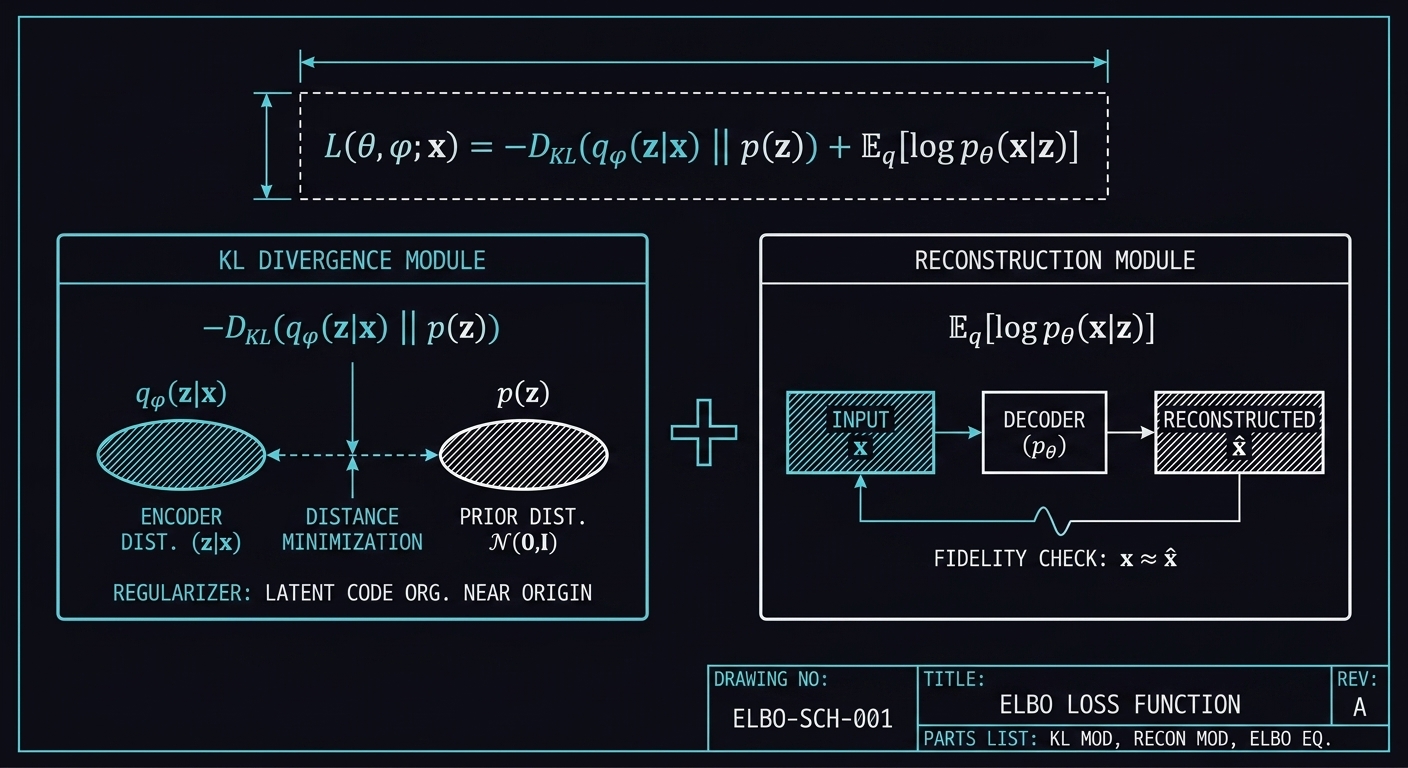 The ELBO has two components: KL Divergence (left) acts as a regularizer keeping latent codes organized near the origin, while Reconstruction (right) ensures the decoder can accurately recreate the input.
The Two Terms Explained
Term 1: KL Divergence (Regularization)
$$-D_{KL}(q_\phi(\mathbf{z}|\mathbf{x}^{(i)}) | p_\theta(\mathbf{z}))$$
What it measures: How different is the encoder’s output distribution from the prior?
Intuition:
- The encoder outputs $q_\phi(\mathbf{z}|\mathbf{x})$ (a distribution, not a point)
- We want this to be close to the prior $p_\theta(\mathbf{z})$ (usually $\mathcal{N}(\mathbf{0}, \mathbf{I})$)
- This regularizes the latent space, preventing the encoder from producing arbitrarily spread-out codes
Why negative?: We’re maximizing the ELBO, and KL is always positive, so we want to minimize KL (hence the negative sign makes it a penalty).
Term 2: Reconstruction (Data Fidelity)
$$\mathbb{E}{q\phi(\mathbf{z}|\mathbf{x}^{(i)})}[\log p_\theta(\mathbf{x}^{(i)}|\mathbf{z})]$$
What it measures: How well can the decoder reconstruct $\mathbf{x}$ from samples of $\mathbf{z}$?
Intuition:
- Sample $\mathbf{z}$ from the encoder’s distribution
- Feed $\mathbf{z}$ to the decoder
- Measure the log-probability of the original $\mathbf{x}$ under the decoder’s output
In practice: This becomes the negative reconstruction error (e.g., MSE for Gaussian decoder, binary cross-entropy for Bernoulli decoder).
The Optimization Objective
Putting it together, we want to maximize:
$$\mathcal{L}(\theta, \phi; \mathbf{x}^{(i)}) = \underbrace{-D_{KL}(q_\phi(\mathbf{z}|\mathbf{x}^{(i)}) | p_\theta(\mathbf{z}))}{\text{Regularization: keep } q \text{ close to prior}} + \underbrace{\mathbb{E}{q_\phi(\mathbf{z}|\mathbf{x}^{(i)})}[\log p_\theta(\mathbf{x}^{(i)}|\mathbf{z})]}_{\text{Reconstruction: decode well}}$$
Or equivalently, minimize:
$$\text{Loss} = D_{KL}(q_\phi(\mathbf{z}|\mathbf{x}) | p(\mathbf{z})) - \mathbb{E}{q\phi(\mathbf{z}|\mathbf{x})}[\log p_\theta(\mathbf{x}|\mathbf{z})]$$
The Problem with Optimization
We want to optimize $\mathcal{L}(\theta, \phi; \mathbf{x}^{(i)})$ with respect to both $\theta$ and $\phi$.
The issue: The gradient with respect to $\phi$ is problematic!
The naïve Monte Carlo gradient estimator:
$$\nabla_\phi \mathbb{E}{q\phi(\mathbf{z})}[f(\mathbf{z})] = \mathbb{E}{q\phi(\mathbf{z})}\left[f(\mathbf{z}) \nabla_{q_\phi(\mathbf{z})} \log q_\phi(\mathbf{z})\right]$$
This is known as the REINFORCE or score function estimator. The paper notes it “exhibits very high variance and is impractical for our purposes.”
Solution: The reparameterization trick (covered in the next section).
Mathematical Derivation of Equation (1)
For completeness, here’s the derivation:
Starting from the definition of KL divergence:
$$D_{KL}(q_\phi(\mathbf{z}|\mathbf{x}) | p_\theta(\mathbf{z}|\mathbf{x})) = \mathbb{E}{q\phi}\left[\log \frac{q_\phi(\mathbf{z}|\mathbf{x})}{p_\theta(\mathbf{z}|\mathbf{x})}\right]$$
Using Bayes’ rule: $p_\theta(\mathbf{z}|\mathbf{x}) = \frac{p_\theta(\mathbf{x}|\mathbf{z})p_\theta(\mathbf{z})}{p_\theta(\mathbf{x})}$
$$D_{KL} = \mathbb{E}{q\phi}\left[\log q_\phi(\mathbf{z}|\mathbf{x}) - \log p_\theta(\mathbf{x}|\mathbf{z}) - \log p_\theta(\mathbf{z}) + \log p_\theta(\mathbf{x})\right]$$
Since $\log p_\theta(\mathbf{x})$ doesn’t depend on $\mathbf{z}$:
$$D_{KL} = \log p_\theta(\mathbf{x}) + \mathbb{E}{q\phi}\left[\log q_\phi(\mathbf{z}|\mathbf{x}) - \log p_\theta(\mathbf{x}|\mathbf{z}) - \log p_\theta(\mathbf{z})\right]$$
Rearranging:
$$\log p_\theta(\mathbf{x}) = D_{KL}(q_\phi | p_\theta) + \underbrace{\mathbb{E}{q\phi}\left[\log p_\theta(\mathbf{x}|\mathbf{z}) + \log p_\theta(\mathbf{z}) - \log q_\phi(\mathbf{z}|\mathbf{x})\right]}_{\mathcal{L}(\theta, \phi; \mathbf{x})}$$
Summary
| Concept | Equation |
|---|---|
| ELBO (Form 1) | $\mathcal{L} = \mathbb{E}_q[-\log q(\mathbf{z} |
| ELBO (Form 2) | $\mathcal{L} = -D_{KL}(q | p(\mathbf{z})) + \mathbb{E}_q[\log p(\mathbf{x} |
| Lower bound property | $\log p(\mathbf{x}) \geq \mathcal{L}$ |
| Tightness | Bound is tight when $q_\phi(\mathbf{z} |